
Blog
Modelling a Phase-Shifting Interferometer
What is a Phase-Shifting Interferometer?
If you have an optics system that requires certain surfaces to be a specific shape (whether it’s flat, spherical, etc.), how would you test that? We can use phase-shifting interferometry to measure the deviation from the intended shape, which is crucial to high-precision manufacturing. This is done by generating multiple interference patterns, called interferograms, against a reference surface for a series of different optical path lengths. From this set of interferograms we can generate the surface sag, or profile, of the test surface.
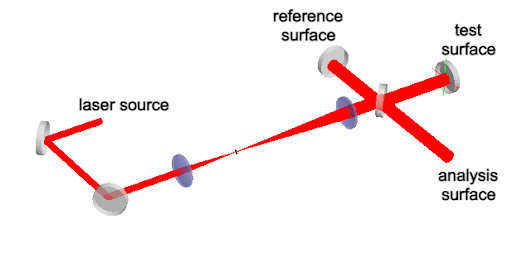
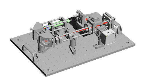
Figure 1. The interferometer example in FRED with only the optics and the rendered ray trace shown.
Interferometer Mechanics
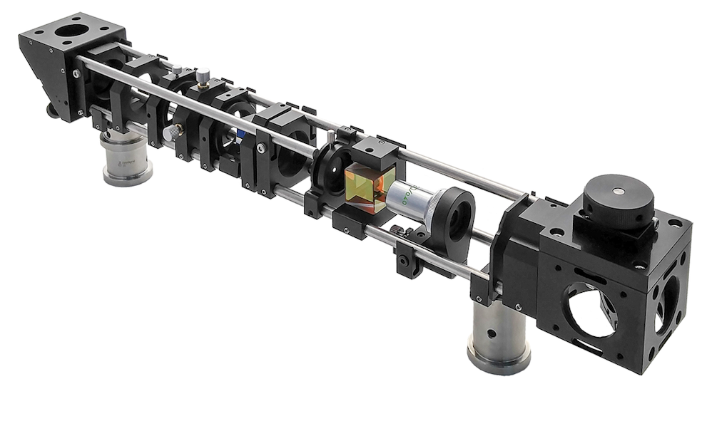
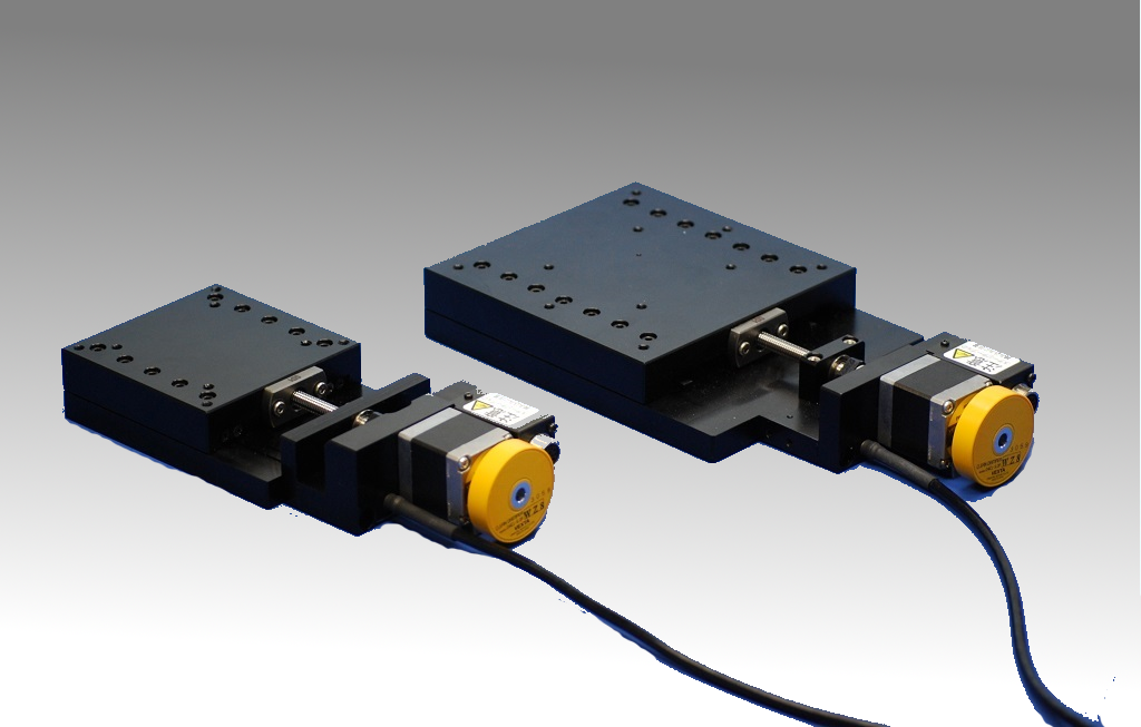
The phase-shifting interferometer is built using commercial off the shelf (COTS) components from OptoSigma. The Optical Cage has some advantages over the Mounting Posts and Dovetail Optical Rails: it is easy to set-up, allowing it to plug directly into the optical bench. It’s easier to transport since the full system is shipped as one unit and it can be imported as a single CAD file into FRED. The Precision Motorized Stage is used for moving the reference mirror by λ/8 (~80 nm) and OptoSigma’s FS-1020UPX motorized stage meets this requirement with a minimum resolution of 1 nm and a positional repeatability of ±2 nm.
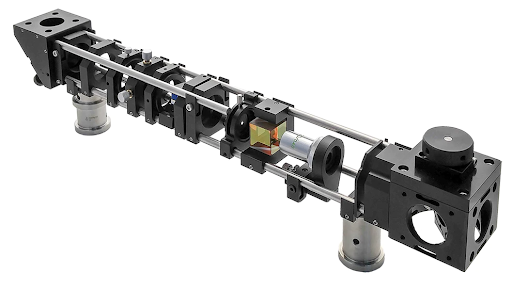
Figure 2. OptoSigma’s Optical Cage (image link)

Figure 3. OptoSigma’s Precision Motorized Stage (image link)
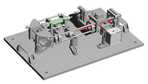
Figure 4. An interferometer example in FRED with OptoSigma mechanics included (grey CAD structures), optics (transparent), and with a ray trace rendered (in red).
Modelling the Phase-Shifting Interferometer
To properly model the analysis described above, we must meet two requirements: (i) an accurate simulation of the propagation of a coherent beam and (ii) our software has to handle a large optical system in a CAD-like interface.
One of FRED’s strongest capabilities is its coherent ray tracing algorithm. The method used is called “Complex Raytracing”. It propagates tiny gaussian beams, which can be used to simulate the propagation of coherent beam(s) in a non-sequential manner. If the beams split off or impinge on an aperture of an optic, that’s handled inherently. Interference and diffraction effects are also all built-in to the algorithm.
Some optical softwares would list all surfaces in the model (optical and mechanical) in a long linear list, which would be painful to manage. FRED uses a CAD-like “tree” to manage both the mechanical and optical parts of the model. This is absolutely essential when dealing with thousands of components and surfaces. FRED has a built-in library of OptoSigma optical parts, but mechanical parts can also be imported from CAD files (STEP, IGES, OBJ).
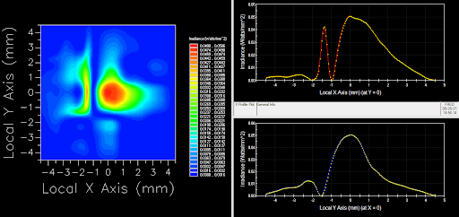
Figure 5. One of the four interferograms generated in the FRED example
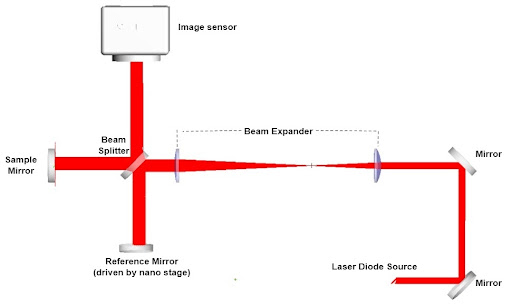
Figure 6. A schematic of the set-up shown in Figure 1 and 2. The Sample Mirror is also referred to as the test surface.
Changing Surface Properties of the Test Surface
In the object tree, all the mechanics and the optics are organized into their own subassemblies. There is another subassembly that we added to our FRED example named “Sag Surface”, which contains several different surface profiles. We start with a flat test surface when the test mirror is initially added to our system, but we can then add a “modifier” surface. The surfaces shown under “Sag Surface” can be quickly added to the test mirror surface to mutate it. For this example, we used the “Freeform” surface type. It is a bicubic mesh where a series of random perturbation points are generated randomly and added to the surface.
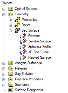
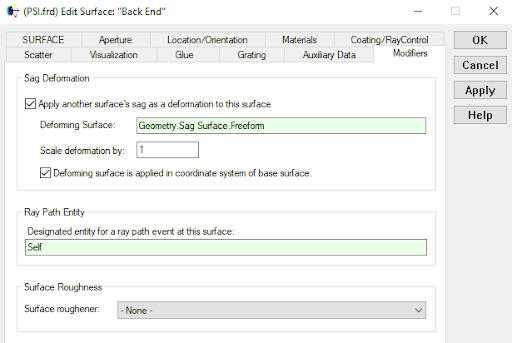
Figure 7. The tree branch in FRED which contains all the surfaces we want to test and the dialog used to change the surface properties of our test surface. With a single click, we can change our “Freeform” surface to another surface we have predefined.
The main idea here is that we can define many different surface types and we can quickly and easily add them to our test surface to analyze them. It is a single setting we change on the test surface, seen in Figure 7, which points to which modifier surface to use.
Interferometry Calculation
The purpose of a phase-shifting interferometer is to analyze the surface profile of the sample mirror, also called the test surface (see Figure 6). The flat reference mirror is moved by a nano-stage system four times, in steps of λ/8 (total path length change of λ/4). Then we recombine the beams and calculate the irradiance for each mirror position onto an image sensor (or an analysis surface in FRED). We can use the four generated interferograms to create what’s called the wrapped phase of the test surface with the following formula:
where Θ(x,y) is the wrapped phase of the test surface and In(x,y) are each of the interferograms with n indicating the changes in the path length in steps of λ/8 (total change of λ/4). From this information we can calculate the sag of the unknown surface profile.
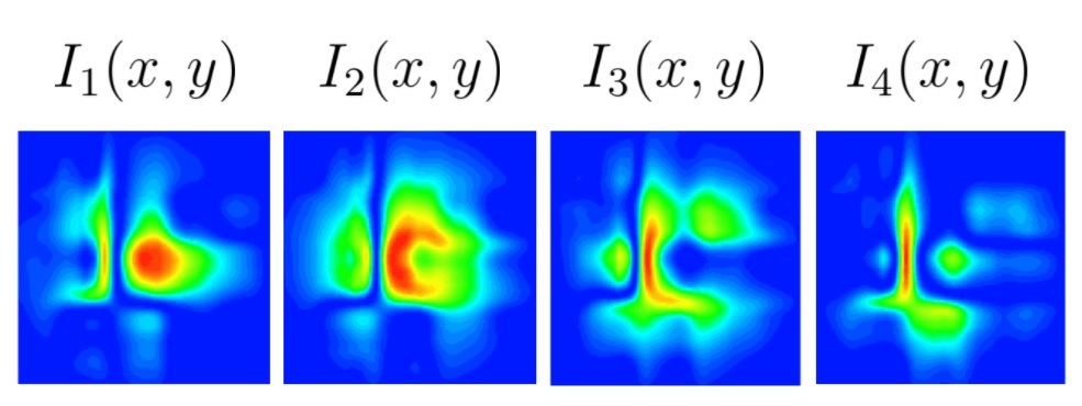
Figure 8. The four interferograms created at every λ/8 step by the reference mirror from this phase-shifting interferometer FRED example. The surface seen here is the “Freeform” type.
To do the interferometry in software, there are two main steps that we automate for ease-of-use. FRED uses the Visual Basic scripting language, which is easy to get started with and powerful.
Calculating the Wrapped Phase
After running our script, it generates the four interferograms, as well as the Wrapped Phase. It stores these results as Analysis Results Nodes (ARNs) in FRED. If we double click on any of them under the Analysis Results branch of the object tree, it will open up the interferograms of the perturbed surface with respect to the distance moved, as seen in Figure 8. The wrapped phase, seen in Figure 9, has a circular aperture which is the laser beam footprint that reaches the test surface. Looking at the aperture size, we can see that the laser beam reaches approximately ± 3 mm.
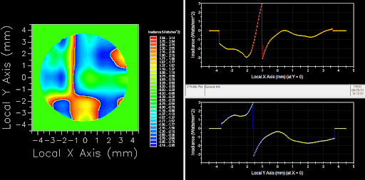
Figure 9. The wrapped phase of our test surface. The surface profiles on the right side of the figure show discontinuities that exist in wrapped phase (-π to π).
Calculating the Surface Sag
We run a second script to unwrap the phase and convert this to sag values in microns. Double clicking on the surface sag ARN gives us the main result of this demonstration (Figure 10). The whole purpose for this interferometer is to provide this result. This is the surface sag, or the deviation from a flat surface, based on this perturbation we used (Freeform), in units of microns. We can see in our result that we range from 0 to half a micron (or 500nm).
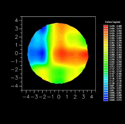
Figure 10. The surface sag of our test surface using the “Freeform” surface assignment. The deviations from flat are given in microns and they range from close to 0 to almost half a micron (or approximately 500 nm).
Summary
Virtual prototyping like this is incredibly useful. In FRED you are able to check if the system you want to design has been set-up correctly; if you have a large enough laser footprint on the test surface; and if there are any issues with misalignment or minor rotation in the stages.
Contact us to request a Demo of FRED or talk through your application needs in more detail.
For information about the OptoSigma parts, please contact:
Axel Haunholter a.haunholter@optosigma-europe.com